Decision Tree
02 May 2018
This time I want to try my hands on using Decision Tree to make predictions. Using Animal Center Outcomes data available from data.world, Animal Center Outcomes from Oct, 1st 2013 to present
or the City of Austin, TX, government website, I am trying to predict whether or not a rescue dog will be adopted based on a selected and simplified list of characteristics. These characteristics include whether the dog was male/female, neutered or spayed/intact, young/old, small dog/big dog breed, and mixed/purebred.
# Simply drop null data, since there are plenty of data points to look at
df = df.drop(df[df['Sex upon Outcome']=='Unknown'].index)

# Get a simplified list of characterisitics
df_simple = df.loc[:,['Animal Type','Sex upon Outcome', 'Outcome Type', 'DateTime','Date of Birth',
                      'Breed']].dropna()

# Concentrate on rescue dogs
df_Dog = df_simple.loc[(df_simple[df_simple['Animal Type'] =='Dog']).index, :]

# Changing data to correct format:

# The predicted variable is 'Outcome Type', and change it to boolean type data
# '1' means adopted, '0' means not adopted
outcome_dict ={'Adoption':1, 'Return to Owner':0, 'Euthanasia':0, 'Transfer':0, 'Died':0, 'Disposal':0,
             'Rto-Adopt':1, 'Missing':0, 'Relocate':0, 'nan':0}
df_Dog['Outcome'] = [outcome_dict[word] for word in df_Dog['Outcome Type']]

# Change date and time to the proper format
df_Dog['DateTimeNew'] = pd.to_datetime(df_Dog.DateTime)
# To get dates only and ignore time values
df_Dog['DateTimeNew'] = pd.DatetimeIndex(df_Dog['DateTimeNew']).normalize()

df_Dog['DateOfBirth'] = pd.to_datetime(df_Dog['Date of Birth'])
df_Dog['DateOfBirth'] = pd.DatetimeIndex(df_Dog['Date of Birth']).normalize()

# To get age(in days) of the dogs at the time of outcome
df_Dog['CalculatedAge'] = df_Dog.DateTimeNew - df_Dog.DateOfBirth
df_Dog['Age'] = df_Dog.CalculatedAge.astype(int)/(1000000000*60*60*24)

# Change other characteristics to boolean type to facilitate data analysis later

smallDog = ['Terrier', 'Chihuahua', 'Miniature','Beagle','Pomeranian',
             'Corgi','Dachshund', 'Apso', 'Shiba','Maltese',
             'Bichon Firse', 'Bulldog', 'Pug']

df_Dog['SmallDog'] = False
for dog in smallDog:
    df_Dog.loc[df_Dog['Breed'].str.contains(dog), 'SmallDog'] = True

df_Dog['Fixed'] = False
df_Dog.loc[df_Dog['Sex upon Outcome'].str.contains('Spayed'), 'Fixed'] = True
df_Dog.loc[df_Dog['Sex upon Outcome'].str.contains('Neutered'), 'Fixed'] = True

df_Dog['Sex'] = 'Male'
df_Dog.loc[df_Dog['Sex upon Outcome'].str.contains('Female'), 'Sex'] = 'Female'
df_Dog['Male'] = True
df_Dog.loc[df_Dog['Sex upon Outcome'].str.contains('Female'), 'Male'] = False

df_Dog['Mix'] = False
df_Dog.loc[df_Dog['Breed'].str.contains('Mix'),'Mix'] = True
Visualizing relations between outcome and variables
import matplotlib.pyplot as plt

x1 = df_Dog[df_Dog['Outcome']==1].Age.values
x0 = df_Dog[df_Dog['Outcome']==0].Age.values

plt.hist(x1, bins=50, histtype='stepfilled', normed=True, color='b', label='Adopted')
plt.hist(x0, bins=50, histtype='stepfilled', normed=True, alpha=0.5, color='r', label='Not adopted')
plt.xlabel("Age(days)")
plt.ylabel("Probability")
plt.legend()
plt.show()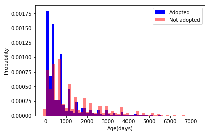
Note: We see that ~300 days is the cut off point where dogs were likely adopted than not.
Therefore I will create the variable ‘Young’ to differentiate between dogs below 300 days old (assigned value of ‘1’) and those above (assigned value of ‘0’).
df_Dog['Young'] = df_Dog.eval('Age < 300')Let’s see how each variable affect outcome (adopted or not)
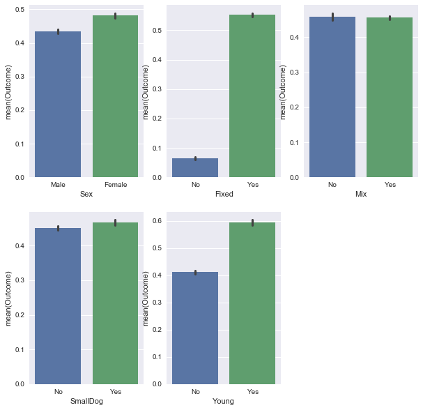
Female dogs, fixed (spayed or neutered), and young dogs are significantly more likely to be adopted, while smaller dog breed are slightly more likely to be adopted. Whether the dog is mixed breed or purebred did not seem to affect outcome… however, let’s see how this one variable interacts with other variables:
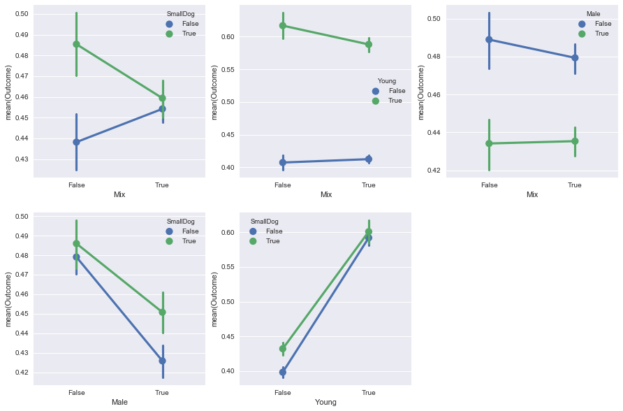
Depending on whether the dog is a small breed, purebred and mixed bred dogs flare differently: for big dogs, mixed bred do better, while for small dogs, purebreds do better.
Making predictions with Decision Tree
from sklearn import tree
from sklearn.model_selection import train_test_split
from sklearn import metrics

x_train, x_test, y_train, y_test = train_test_split (df_Dog_X, df_Dog_y, test_size= 0.3, random_state = 42)

modelDTC_Dog = tree.DecisionTreeClassifier(criterion='gini')
modelDTC_Dog.fit(x_train, y_train)
predictedDTC_Dog = modelDTC_Dog.predict(x_test)

print('Accuracy: ', metrics.accuracy_score(y_test, predictedDTC_Dog))

# To see samples of predicted results, compared with real outcome:
print('predicted: ', list(predictedDTC_Dog[0:20]))
print('true: ', list(y_test[0:20]))
Accuracy: 0.654023536896
predicted: [0, 0, 0, 1, 0, 0, 0, 1, 0, 1, 0, 1, 1, 1, 0, 0, 0, 0, 1, 1]
true: [0, 0, 0, 1, 1, 0, 0, 1, 1, 0, 0, 1, 1, 1, 0, 0, 0, 1, 1, 1]
To visualize the Decision Tree
tree.export_graphviz(modelDTC_Dog, feature_names=df_Dog_X.columns,
                         out_file='AustinDTCDogtreeTestData.dot')
I ran into trouble trying to see the tree within Python notebook, but the webgraphviz website made it really easy to see it in their browser.
The resultant tree is a bit complicated. But we can see that dogs who are fixed and young have the best chance of getting adopted.
