Using Seaborn Heatmap

After talking to my friend (the one who gave me her neurite growth rate data to play with), she suggested to improve the presentation a little. So, as a continuation to Jan18’s ‘How to Visualize Biological Data Using a Heatmap’, here’s the main points of our modification:

1. Instead of a linear scale consisting of neurite growth rate data used as is, we categorized them into ‘fast retract’, ‘slow retract’,’very slow retract’,’very slow growth’, ‘slow growth’, ‘fast growth’. This can be done using pandas’ cut function.

pandas.cut(x, bins, right=True, labels=None, retbins=False, precision=3, include_lowest=False)

1. To plot heatmap, numerical data are needed, so the above categorical data are converted into numbers. This can be done using pandas’ map function.

Series.map(arg, na_action=None)

Step 1

The dataset contained null data, because (1) in live-imaging, not all cells survived for exactly the same amount of time. My friend kept the cells alive for as long as possible, but some died or became non-responsive faster than others; (2) I find that empty lines within the dataset give good visual separation between each type of cells - wildtype, transgenicA, transgenicB, etc. So here I’m going to fill NaN data with an abnormally large value (10), that’s not found within the dataset:

import pandas as pd
import matplotlib.pyplot as plt
data = pd.read_excel('Neurite growth rate file')

data_fillna = data.fillna(10)
data_categorized = data_fillna.copy()
for col in data_categorized.columns:
    data_categorized[col] = pd.cut(data_fillna[col], \
      bins=[-7,-4,-2,0,2,4,7], \
      labels=['fast retract', 'slow retract','very slow retract','very slow growth',\
      'slow growth', 'fast growth'])

The code divides the data into 6 categories corresponding to:

-7 to -4: ‘fast retract’
-4 to -2: ‘slow retract’
etc.

By default, the bins include the rightmost edge, so in fact it means,

(-7, 2]: ‘fast retract’
(-4, -2]: ‘slow retract’
etc.

Step 2

Now I’m going to use the map function change the categories to numbers so that Python can read it and plot it out as a heatmap

color_map = {'fast retract':1, 'slow retract':2,'very slow retract':3,'very slow growth':4, 'slow growth':5, 'fast growth':6}
for col in data_categorized.columns:
    data_categorized[col] = data_categorized[col].map(color_map)

Step 3

Now to plot the heatmap, I choose the categorical color scheme ‘Vega10’. Also, as a result from the categorization step (Step 1), data points that are not in the dictionary (i.e. neurite retraction slower than -7, and growth faster than 7) are converted to NaN data. So I’m going to fillna with a number (7.5) that is not one of those used in the map function (1,2,3,4,5,6), so that when the data are ploted as a heatmap, its background color is different from the colors used for the data points.

u = np.linspace(0, 22, 23)
v = np.linspace(0, 116, 117)
X,Y = np.meshgrid(v,u)
Z = data_categorized.fillna(7.5) 
plt.pcolor(X, Y, Z, cmap=plt.get_cmap('Vega10'))
plt.subplots_adjust(left=0, right=2, bottom=0, top=1.5)
plt.ylabel('Animal')
plt.yaxis=dict(autorange='reversed')
plt.xlabel('Time')
yindex = range(0,22)
ylabel = list(data_categorized.index)
plt.yticks(yindex, ylabel, va = 'bottom')
plt.colorbar()
plt.show()

Here’s the resultant heatmap:

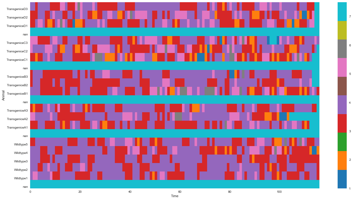
It looks okay, but,

let’s try with Seaborn,

import seaborn as sns

plt.figure(figsize = (16,10)) 
image = sns.heatmap(data_categorized, annot=False, annot_kws={"size": 10}, xticklabels=5, cmap=plt.get_cmap('Vega10')) 
sns.plt.show()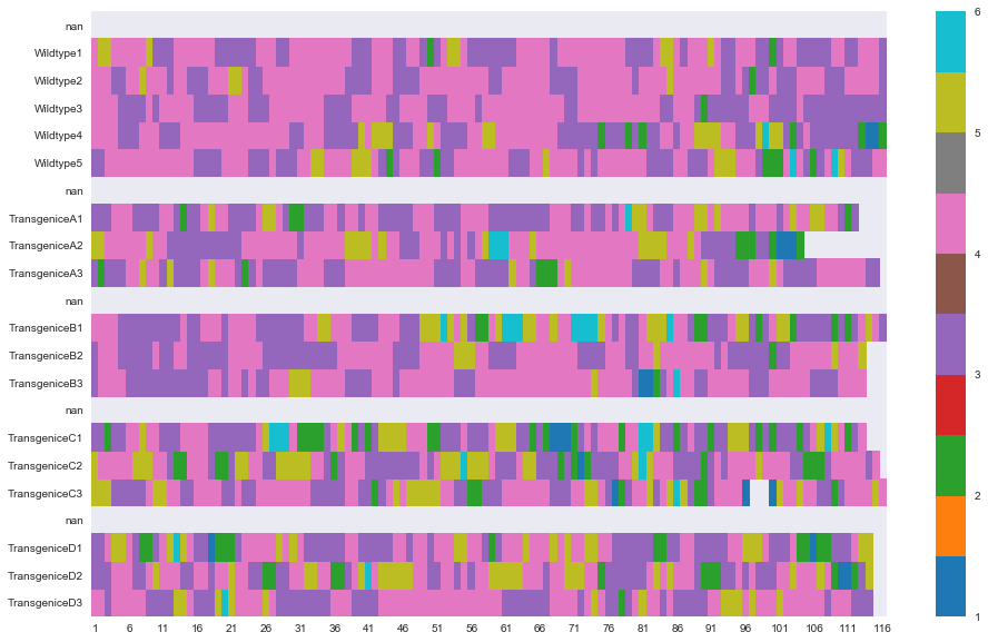

With Seaborn, I don’t need to specify background color using ‘fillna’. It just automatically assigns a nice neutral color! Sweet!